CPU 인터커넥트 설계 지표
개요
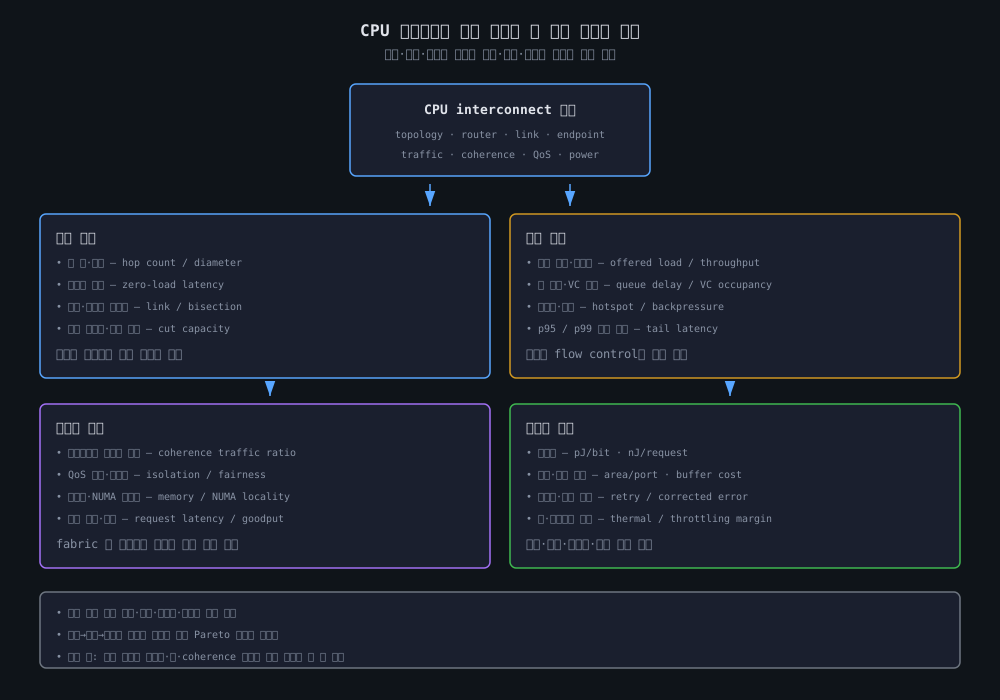
CPU 인터커넥트는 코어, cache slice, home agent, memory controller, I/O agent를 연결하면서 요청과 응답을 운반한다. 코어 수와 에이전트 수가 증가하면 링크 속도 하나만 높이는 것으로는 충분하지 않다. 어떤 노드 사이의 경로가 긴지, 네트워크를 둘로 나눴을 때 절단면의 용량이 충분한지, 특정 링크에 트래픽이 몰리는지, 지연에 민감한 요청이 다른 트래픽에 밀리는지를 함께 측정해야 한다.
이 문서의 지표는 구조·동작·시스템의 세 계층으로 나누고, 전력·면적·신뢰성·열은 비기능 관점으로 별도 관리한다. 구조 지표는 topology와 경로의 잠재적 한계를, 동작 지표는 실제 큐·중재·flow control의 상태를, 시스템 지표는 coherence·QoS·메모리 service까지 포함한 제품 수준의 결과를 다룬다. 따라서 hop latency가 낮아도 bisection bandwidth가 부족하거나, peak bandwidth가 높아도 queueing과 coherence traffic 때문에 tail latency가 클 수 있다.
핵심 개념
1. 측정 경계와 단위
먼저 측정 대상이 network-only인지, endpoint와 memory controller를 포함한 fabric transaction인지 정해야 한다. 예를 들어 라우터 사이의 flit 지연은 network latency이고, 코어의 cache miss부터 data 반환까지는 endpoint queue, coherence lookup, DRAM service time이 포함된 request latency다. 두 값을 섞으면 topology 변경의 효과를 잘못 해석할 수 있다.
| 구분 | 대표 단위 | 의미 | 포함 범위 |
|---|---|---|---|
| 시간 | cycle, ns | 한 요청 또는 패킷의 지연 | 정의에 따라 router/link만 또는 endpoint·service 포함 |
| 용량 | bit/s, byte/s, flit/cycle | 링크 또는 cut이 이론적으로 운반할 수 있는 양 | link width, frequency, encoding, 방향성 반영 |
| 부하 | flit/cycle, request/s | 네트워크에 주입하는 offered load | source·class·packet size를 함께 기록 |
| 사용률 | %, busy cycles | 링크·VC·buffer가 실제로 사용된 비율 | 시간 평균과 최대 hotspot을 구분 |
| 에너지 | pJ/bit, nJ/request | 전송 또는 요청 처리당 에너지 | wire, router, buffer, PHY, retry 경계 명시 |
| 면적 | mm², mm²/port | 인터커넥트 구현에 필요한 물리 비용 | router, buffer, link, clock·전원 배선 포함 여부 |
2. Hop latency와 경로 길이
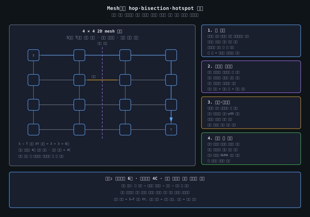
hop count는 source와 destination 사이에서 통과하는 링크 또는 router의 수다. 정적 XY routing에서는 source와 destination의 좌표 차이로 최소 경로를 계산할 수 있지만, adaptive routing이나 congestion 우회가 있으면 실제 hop 수는 실행마다 달라질 수 있다. 링에서는 방향 선택에 따라 경로가 달라지고, die-to-die 링크를 하나의 hop으로 셀지 PHY와 adapter를 분리해 셀지도 정해야 한다.
network diameter는 모든 노드 쌍의 최단 경로 중 최댓값으로, topology가 제공하는 최악-case 경로 길이를 요약한다. 평균 hop count가 비슷한 두 구조라도 diameter와 경로 분포가 다르면 원격 요청의 tail latency가 달라질 수 있다.
네트워크 경로의 기본 지연은 다음처럼 분해할 수 있다.
L_network = L_injection + Σ(L_router_i + L_link_i) + L_serialization + L_queue
L_request = L_network + L_home_or_coherence + L_memory_or_device + L_return
L_injection: endpoint가 packet/flit을 만들고 ingress queue에서 전송을 시작하기까지의 시간L_router: route computation, VC/switch arbitration, crossbar traversal에 걸리는 시간L_link: 링크를 건너는 물리적·논리적 전달 시간L_serialization: 링크 폭보다 packet이 클 때 여러 flit으로 나누어 전송하는 시간L_queue: 입력 buffer, VC, output port에서 경쟁 때문에 기다린 시간
설계 초기에는 zero-load latency와 loaded latency를 분리해 측정해야 한다. zero-load 값은 topology와 pipeline의 기본 비용을 보여주고, 두 값의 차이는 queueing·arbitration·backpressure가 추가한 비용을 보여준다. 평균 hop 수만 보고 최악 경로와 높은 백분위 지연을 생략하면 hotspot을 놓칠 수 있다.
3. Link bandwidth와 bisection bandwidth
단일 링크의 이상적인 raw capacity는 구현 방식에 따라 다음과 같이 근사할 수 있다.
C_link = link_width_bits × transfers_per_cycle × link_frequency × efficiency
여기서 efficiency는 line coding, framing, CRC/retry, flow-control credit, protocol header 등으로 실제 payload에 쓰이지 않는 비율을 반영한다. full-duplex 링크라면 방향별 capacity와 양방향 aggregate를 분리해서 기록해야 한다.
Bisection bandwidth는 네트워크 노드를 거의 같은 크기의 두 집합으로 나눌 때, 두 집합 사이를 가로지르는 cut의 capacity를 보는 지표다. 그래프 G=(V,E)와 링크 용량 C_e에 대해 이상적인 정의는 다음과 같이 쓸 수 있다.
B_bisection = min over balanced S of Σ(C_e for e in cut(S, V-S))
이 값은 많은 노드가 반대편 노드와 동시에 통신하는 all-to-all 또는 균등한 remote-access workload에서 구조적 병목을 찾는 데 유용하다. 그러나 실제 sustained throughput은 endpoint 주입 능력, routing, arbitration, packet header, coherence와 memory-controller service capacity 때문에 이론값보다 낮다. 따라서 peak link rate, aggregate link capacity, bisection capacity, measured delivered throughput을 같은 숫자로 취급하면 안 된다.
4. Offered load, throughput, saturation
네트워크에 넣으려는 양을 offered load, 목적지에 성공적으로 도착한 양을 delivered throughput이라고 구분한다. offered load를 조금씩 증가시킬 때 delivered throughput이 선형으로 늘다가 더 이상 늘지 않고 지연이 급격히 증가하는 지점을 saturation point로 본다. 링크 사용률이 100%가 되기 전에 endpoint나 특정 output port가 먼저 병목이 될 수 있으므로 전체 평균 사용률만으로 saturation을 판정해서는 안 된다.
다음 지표를 한 실험에서 함께 수집한다.
| 지표 | 계산 예 | 읽는 방법 |
|---|---|---|
| Injection rate | 주입 flit 수 / cycle / source | source가 fabric에 제공한 부하 |
| Delivered throughput | 도착한 payload / 시간 | 실제 유효 데이터 처리량 |
| Link utilization | busy cycles / 관찰 cycles | 평균보다 max·분포가 중요 |
| Packet latency | 도착 timestamp - 주입 timestamp | packet size와 traffic class별로 분리 |
| Saturation load | 지연 상승 또는 처리량 plateau의 부하 | topology·routing·buffer 설정에 종속 |
| Goodput | 유효 payload / 전체 전송량 | header·retry·coherence control 비용을 제외한 결과 |
5. Congestion과 hotspot
혼잡은 단순히 링크 사용률이 높은 상태가 아니라, 경쟁하는 flit이 buffer와 arbitration을 점유하여 다른 요청의 진행을 늦추는 상태다. 특히 여러 source가 하나의 memory controller, LLC home, ring segment 또는 mesh 링크를 공유하는 hotspot workload에서 평균값과 최대값의 차이가 커진다.
- Queue occupancy: input buffer, VC, output queue가 얼마나 차 있는지 기록한다.
- Queueing delay: flit이 유효하지만 전송 승자를 기다린 시간이다.
- Backpressure: downstream credit 또는 ready가 부족해 upstream 주입이 멈춘 횟수와 지속 시간을 측정한다.
- Hotspot ratio: 최대 link utilization을 평균 link utilization으로 나눈 값이다.
- Fairness: source별 throughput 또는 latency 편차를 확인한다. 평균 처리량이 같아도 한 source가 starvation을 겪을 수 있다.
max link utilization, max VC occupancy, p99 latency를 함께 보면 평균 throughput만으로는 보이지 않는 congestion을 찾을 수 있다. virtual channel을 추가하면 traffic class를 분리할 수 있지만 buffer와 arbitration 면적, deadlock 회피 검증 부담도 증가한다.
6. QoS와 tail latency
CPU demand, DMA, I/O, coherence control은 서로 다른 지연 요구를 가진다. QoS 평가에서는 평균 latency보다 p95·p99·p99.9와 같은 tail latency, class별 최소 서비스량, priority inversion, starvation을 봐야 한다. 한 class의 평균 latency가 낮아도 다른 class의 tail이 무한히 늘면 격리가 실패한 것이다.
| 질문 | 필요한 측정 |
|---|---|
| 지연 민감 CPU 요청이 보호되는가? | traffic class별 p50/p95/p99 latency |
| bandwidth class가 링크를 독점하는가? | class별 delivered throughput·link share |
| 우선순위가 starvation을 만드는가? | 최대 대기 cycle·최소 service rate |
| 경로가 공정한가? | source별 latency/throughput 분포 |
| congestion이 어느 계층에서 시작되는가? | ingress queue, VC, router, egress queue 시계열 |
QoS 정책은 단순한 priority 숫자만의 문제가 아니다. virtual network, VC, credit, age-based arbitration, rate limiter를 함께 설계해야 하며, coherence acknowledgement처럼 낮은 대역폭이지만 진행이 막히면 시스템 전체를 멈출 수 있는 control traffic도 별도 고려해야 한다.
7. Coherence traffic과 메모리 트래픽
coherent CPU에서는 data packet 외에 snoop, directory lookup, invalidate, ownership, acknowledgement, data forwarding 메시지가 fabric을 사용한다. 따라서 유효한 data byte만 세는 bandwidth와 fabric이 실제로 운반한 총 byte/flit을 분리해야 한다.
| 지표 | 의미 |
|---|---|
| Coherence message rate | 요청당 snoop·directory·invalidate·ack 수 |
| Coherence traffic ratio | coherence 제어·forwarding traffic / 전체 fabric traffic |
| Sharing-induced invalidation | 공유 line에 대한 소유권 전환과 invalidate 빈도 |
| Directory occupancy | home agent가 유지하는 line metadata 사용량 |
| Forwarding ratio | memory가 아니라 다른 cache가 데이터를 공급한 비율 |
| Remote access ratio | 로컬 home·memory가 아닌 경로로 처리된 요청 비율 |
예를 들어 공유 cache line이 자주 쓰이면 data payload는 작아도 ownership 전환과 invalidate가 링크를 점유할 수 있다. 이때 mesh의 nominal bisection bandwidth보다 coherence traffic이 만드는 control-message queue와 ordering dependency가 성능을 제한할 수 있다. 캐시 일관성 프로토콜의 상태 전이와 메모리 인터커넥트의 flow control을 함께 봐야 하는 이유다.
8. 전력, 면적, 신뢰성
인터커넥트는 장거리 wire, router pipeline, crossbar, input buffer, clock distribution, PHY가 전력과 면적을 소비한다. pJ/bit는 이동 효율을 보는 유용한 지표지만, 짧은 control packet의 고정 router 비용과 retry·replay 비용이 빠질 수 있으므로 nJ/request와 같이 봐야 한다.
- Dynamic energy: 토글하는 wire, router, buffer, arbitration의 switching energy
- Static/leakage energy: 유휴 router, PHY, SRAM buffer의 leakage
- Area per port: 포트 수와 virtual channel·buffer 깊이에 따른 router 면적
- Wire cost: 긴 global wire의 repeater, 층간 배선, congestion 완화용 routing resource
- Retry overhead: CRC 오류와 재전송으로 증가한 energy와 latency
- Thermal density: 링크와 PHY가 집중된 영역의 열 밀도와 throttling 영향
die-to-die와 socket link에서는 on-die wire와 달리 PHY, lane training, CRC, retry, power state가 측정 경계에 들어온다. UCIe와 같은 표준은 package-level physical layer와 adapter, protocol, software stack을 함께 다루지만, 그 위의 CPU coherence 정책이나 제품별 routing을 자동으로 정해 주지는 않는다.
비교/분석
토폴로지별 지표 프로파일
| 토폴로지 | hop latency 경향 | bisection bandwidth | hotspot 위험 | 비용과 적합성 |
|---|---|---|---|---|
| 공유 bus | 짧을 수 있으나 arbitration 대기 증가 | 공유 매체 하나에 집중 | 매우 높음 | 소규모 agent, 단순 제어에 유리 |
| Ring | 노드 수와 방향 선택에 따라 증가 | 링크 수와 ring 방향에 제한 | 특정 segment·home에 집중 가능 | 중간 규모에서 낮은 router 비용 |
| 2D mesh | 위치에 따라 여러 hop | 균등 mesh는 cut 용량을 예측하기 쉬움 | 비균등 endpoint 배치와 hotspot에 민감 | 다중 코어·LLC·MC 확장에 유리 |
| Crossbar | 직접 경로로 낮은 경로 지연 | 중앙 switch가 병목이 될 수 있음 | 포트 경쟁이 중앙 집중 | 소수 고대역폭 endpoint에 적합 |
| 계층형·chiplet fabric | 계층 경계마다 지연 편차 | die 내부 cut과 die-to-die link가 함께 제한 | home·IOD·PHY 경계에 집중 | 공정 혼합·수율 이점, 검증·패키지 비용 증가 |
표의 경향은 동일한 링크 폭, frequency, traffic model을 가정한 구조적 비교일 뿐 제품 성능 순위가 아니다. 실제 비교에서는 cache sharing, request size, read/write 비율, memory-controller mapping, NUMA placement, routing algorithm, buffer depth를 고정해야 한다.
설계 질문과 지표 매핑
| 설계 질문 | 1차 지표 | 함께 확인할 지표 | 잘못된 결론의 예 |
|---|---|---|---|
| 코어 수를 더 늘릴 수 있는가? | bisection bandwidth, max hop | area/port, power/bit, coherence ratio | 링크 수가 늘었으니 확장 가능하다고 판단 |
| cache miss 응답을 빨리할 수 있는가? | zero-load·loaded latency | p99, memory service time, queue delay | 평균 hop만 보고 latency 개선을 주장 |
| DMA가 CPU를 방해하지 않는가? | class별 throughput share | QoS tail, VC occupancy, starvation | 전체 평균 latency만 비교 |
| 특정 LLC/home이 병목인가? | per-link·per-agent utilization | queue occupancy, request concentration | 평균 utilization으로 hotspot을 숨김 |
| die를 분리해도 이득인가? | payload bandwidth, nJ/bit | PHY overhead, retry, thermal, remote ratio | raw die-to-die rate를 end-to-end 성능으로 간주 |
| 전력 예산 안에서 동작하는가? | pJ/bit, nJ/request | static power, traffic mix, throttling | payload bit만 세고 control·retry를 제외 |
단순 계산 예시
다음은 특정 제품 수치가 아닌 단위와 절차를 보여주기 위한 가정이다. 8×8 mesh의 각 방향 링크가 64 bit 폭이고 2 GHz에서 cycle당 한 번 전송하며, protocol overhead를 일단 무시한다고 하자.
C_link = 64 bit × 2 Gtransfer/s = 128 Gbit/s = 16 GB/s
vertical bisection capacity = 8 crossing links × 16 GB/s = 128 GB/s
한 corner node에서 반대 corner node로 XY routing을 사용하면 최소 경로는 7 + 7 = 14 링크다. 반면 중앙에 memory controller를 두고 여러 코어가 동시에 접근하면 모든 요청이 같은 destination-side links와 egress queue를 공유할 수 있다. 따라서 128 GB/s라는 cut capacity가 있어도 endpoint 주입 폭, memory service capacity, arbitration, coherence control이 더 작은 병목이면 end-to-end throughput은 그보다 낮다.
이 예시를 실험으로 바꿀 때는 다음을 고정해야 한다.
- 링크가 full-duplex인지, 16 GB/s가 방향별인지 aggregate인지 기록한다.
- control packet과 data packet의 크기, flit size, header·retry overhead를 명시한다.
- uniform random, transpose/all-to-all, single hotspot, nearest-neighbor를 별도 workload로 실행한다.
- 평균 latency뿐 아니라 source별 p99, per-link max utilization, delivered throughput을 저장한다.
- coherence traffic과 memory controller queue를 포함한 realistic trace로 결과를 재검증한다.
동작 원리
1단계: 트래픽과 측정 계획 정의
먼저 system boundary와 목표를 정한다. on-die router만 비교할지, die-to-die PHY와 memory controller까지 포함할지 결정하고, CPU demand·coherence·DMA·I/O를 traffic class로 나눈다. packet size, read/write 비율, source-destination matrix, working-set locality, burstiness, warm-up과 측정 구간을 문서화해야 한다.
최소 실험군은 네 가지가 유용하다.
- Uniform random: 평균 경로와 평균 용량의 baseline
- Nearest neighbor: 짧은 경로와 local traffic 효율 확인
- Transpose 또는 all-to-all: bisection과 global congestion 확인
- Single/multiple hotspot: home agent, LLC slice, memory controller 집중 부하 확인
2단계: 요청 주입과 fabric traversal
endpoint가 요청을 packet 또는 flit으로 만들면 ingress queue에 넣는다. router는 route computation, VC selection, switch allocation, switch traversal, link traversal을 수행하며, downstream credit가 없으면 전송을 보류한다. 이때 각 단계의 timestamp를 남기면 total latency를 다음 부분으로 나눌 수 있다.
total latency
  = endpoint injection
  + router/link traversal
  + arbitration and queueing
  + coherence or home-agent service
  + memory/I/O service
  + response traversal
cycle-accurate NoC 모델은 이 분해에 적합하다. 예를 들어 gem5 Garnet 2.0은 router의 buffer write, route compute, switch allocation, VC selection, switch traversal, link traversal을 별도 단계로 모델링하고, topology별 router/link delay와 virtual channel을 설정할 수 있다. 이 모델에서 관측한 network latency를 실제 silicon의 cache-miss latency와 동일시하지 말고, 모델 boundary를 함께 보고해야 한다.
3단계: 혼잡과 QoS 관측
offered load를 낮은 값에서 saturation 근처까지 단계적으로 올리면서 다음 시계열을 기록한다.
- per-link busy cycle과 방향별 utilization
- input/output queue occupancy와 VC별 credit
- route별 hop count와 queueing delay
- traffic class별 delivered throughput과 latency percentile
- backpressure 발생 횟수와 지속 cycle
- arbitration winner, age, starvation 또는 retry 이벤트
평균 queue occupancy가 낮아도 짧은 시간의 burst가 p99 latency를 만들 수 있다. 그러므로 시간 평균과 함께 최대값, percentile, burst window를 저장해야 한다. priority 정책을 바꿀 때는 우선순위 class의 latency만 낮아졌는지, 낮은 우선순위 class가 starvation에 빠졌는지를 동시에 확인한다.
4단계: coherence와 메모리 경로 결합
cache miss trace를 fabric trace와 결합하면 다음 순서로 병목을 분리할 수 있다.
- miss가 발생한 core와 요청 주소의 home agent를 확인한다.
- directory lookup, snoop, invalidate, ownership response의 message 수를 센다.
- data가 다른 cache에서 forward되었는지 memory controller에서 왔는지 구분한다.
- home agent와 memory controller의 queue 대기 시간을 network queue 대기와 분리한다.
- local/remote home과 NUMA placement를 바꿔 latency·throughput 민감도를 비교한다.
이 과정을 거치면 fabric이 느리다는 관찰을 특정 cut의 congestion, coherence amplification, remote memory service, endpoint injection 제한 중 하나로 좁힐 수 있다.
5단계: 전력·면적·신뢰성 모델 결합
성능이 같은 두 topology를 비교할 때는 link toggle, router activity, buffer read/write, clock, PHY, retry를 traffic trace와 연결한다. total energy / delivered payload bit는 payload 관점의 효율이고, total energy / completed request는 control traffic과 고정 비용을 포함한 시스템 관점의 효율이다. die-to-die라면 corrected error, retry rate, lane degradation, link retraining과 thermal throttling도 같은 구간에서 기록한다.
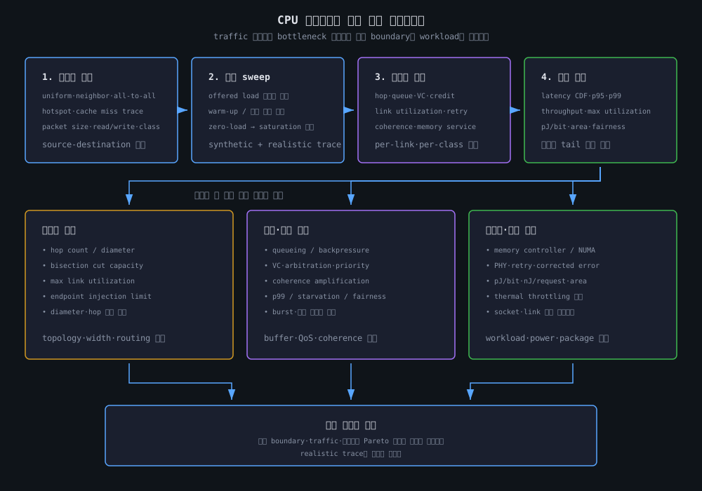
6단계: 결과 판정과 sensitivity analysis
한 개의 종합 점수로 topology를 고르기보다 설계 목표별 Pareto frontier를 작성한다. 예를 들어 ring은 면적과 zero-load cost가 유리하지만 core 수 증가 시 hop·hotspot이 불리할 수 있고, mesh는 parallel path와 bisection 측면에서 유리하지만 router·wire·buffer 비용이 증가한다. chiplet은 die 크기와 공정 재사용의 이점이 있지만 package link와 remote locality가 새 경계를 만든다.
다음 파라미터를 하나씩 바꾸는 sensitivity analysis가 유용하다.
- router pipeline latency와 link latency
- link width, frequency, full/half-duplex 방향성
- buffer depth와 virtual channel 수
- deterministic routing과 adaptive routing
- arbitration의 priority, round-robin, age 정책
- coherence sharing 비율과 home-agent 배치
- source locality, memory mapping, NUMA placement
- packet size, burst length, read/write 비율
장단점
| 장점 | 단점 및 주의점 |
|---|---|
| hop·cut·queue를 분리해 구조적 병목을 조기에 찾을 수 있음 | metric boundary를 잘못 정하면 서로 다른 비용을 비교하게 됨 |
| offered load sweep으로 saturation과 tail latency를 볼 수 있음 | synthetic traffic 결과가 실제 coherence trace를 대표하지 않을 수 있음 |
| per-link·per-class 지표로 hotspot과 QoS 침해를 드러낼 수 있음 | vendor silicon counter의 명칭과 집계 범위가 제품마다 다름 |
| power·area·retry를 throughput과 함께 Pareto 비교할 수 있음 | 초기 power/area 모델은 physical implementation 오차가 큼 |
| gem5 Garnet·BookSim 등으로 설계 공간을 반복 탐색할 수 있음 | simulator의 router·protocol 모델이 실제 fabric과 다를 수 있음 |
| chiplet과 socket 경계를 포함한 end-to-end 분석 가능 | package PHY, thermal, NUMA, OS placement까지 검증 범위가 넓어짐 |
가장 흔한 오류는 peak bandwidth를 sustained bandwidth로, 평균 latency를 tail latency로, network-only latency를 memory access latency로 바꾸어 말하는 것이다. 결과를 공유할 때는 topology, link width/frequency, packet/flit size, routing, buffer/VC, traffic matrix, coherence 포함 여부를 함께 적어야 재현성이 생긴다.
관련 기술
- CPU Fabric 아키텍처 개요: CPU fabric의 topology, 계층, coherence와 QoS 구성
- 메모리 인터커넥트: bus, ring, mesh, NoC와 flow control
- 캐시 일관성 프로토콜: snoop, directory, MESI/MOESI 트래픽
- NUMA 아키텍처: socket locality와 remote-memory 비용
- 캐시 일관성 MESI/MOESI: coherence 상태와 directory metadata
- 메모리 컨트롤러: queue, scheduling, QoS와 DRAM service time
- 카운터/모니터링: PMU, sampling, telemetry 기반 관측
- UCIe 칩렛 인터커넥트: die-to-die package boundary와 PHY/adapter
- PCIe Gen5/Gen6: 외부 link의 encoding·retry·flow-control 경계
참고 문헌 및 표준
- L. Benini and G. De Micheli, “Networks on Chips: A New SoC Paradigm,” IEEE Computer, 2002, doi:10.1109/2.976921: NoC의 구조와 설계 문제를 정리한 초기 연구.
- William J. Dally and Brian Towles, Principles and Practices of Interconnection Networks, Morgan Kaufmann, book page: interconnection network의 topology, routing, flow control, performance 분석.
- Nan Jiang et al., “A Detailed and Flexible Cycle-Accurate Network-on-Chip Simulator,” ISPASS, 2013, BookSim 2.0 repository: cycle-accurate topology·routing·router 실험 도구.
- gem5, Garnet 2.0 documentation: router pipeline, virtual channel, credit flow control과 topology parameter 모델.
- Arm, Neoverse CMN-700: Scalable Mesh for Systems: coherent mesh와 확장 가능한 system IP의 공개 개요.
- UCIe Consortium, UCIe Specifications: package-level die-to-die physical layer, adapter, protocol, software stack과 세대별 기능.
핵심 정리
- CPU 인터커넥트 평가는 hop latency 하나가 아니라 bandwidth, bisection, congestion, QoS, coherence traffic, power와 area를 함께 측정해야 한다.
peak link rate,bisection capacity,sustained throughput은 서로 다른 지표이며, endpoint·protocol·memory service 비용 때문에 값이 달라진다.- 평균 latency보다 per-link hotspot, queue occupancy, p95/p99 tail latency와 class별 최소 서비스량이 실제 병목과 QoS 실패를 더 잘 드러낸다.
- coherence와 NUMA를 제외한 synthetic network 결과는 end-to-end CPU 성능을 직접 의미하지 않으므로 realistic trace와 결합해 검증해야 한다.
- 좋은 topology는 절대적으로 정해지지 않으며, 목표한 지연·처리량·전력·면적·신뢰성의 Pareto 균형과 향후 확장 계획으로 선택한다.